Traverse Closure Explained: How Surveyors Catch Measurement Errors Before They Compound
A closed survey traverse should return exactly to its starting point — it never does. The gap, and how surveyors quantify and correct it, is the real math here.
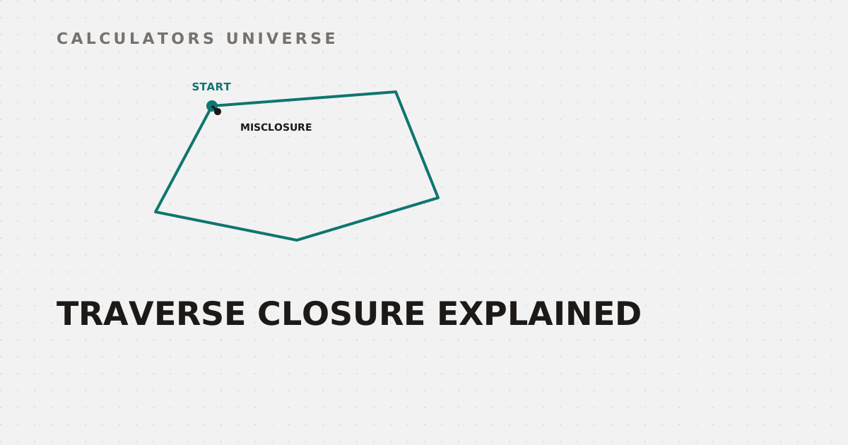
Traverse Closure Explained: Catching Errors Before They Compound
A closed traverse — a survey that walks from a known point, leg by leg, and returns to that same starting point — should mathematically arrive back exactly where it began. It never does. Every bearing and distance measurement carries a tiny bit of error, and by the time the last leg closes the loop, those small errors have accumulated into a real, measurable gap. How surveyors quantify that gap, judge whether it’s acceptable, and correct for it is the actual math behind trustworthy fieldwork.
The Linear Misclosure: Where the Traverse “Should” Have Ended
Each traverse leg is broken into a latitude (its north-south component) and a departure (its east-west component). For a perfectly closed traverse, the sum of all latitudes and the sum of all departures around the loop should each equal exactly zero — you end up back at your start. In practice, both sums come out slightly nonzero, forming a small linear misclosure vector.
The traverse should return to exactly the starting point — the small gap is the linear error of closure
The magnitude of that gap is the Linear Error of Closure (LEC): LEC = √(ΣLat² + ΣDep²). On its own, that number doesn’t tell you much — a 0.3-meter gap is excellent on a 50km traverse and alarming on a 200-meter one. Compute the exact misclosure and adjusted coordinates for your own field data with the Traverse Closure & Bowditch Adjustment Calculator.
Precision Ratio: Turning an Error Into a Quality Grade
To make the closure error meaningful, surveyors divide it by the traverse’s total perimeter length to get a precision ratio, expressed as 1:X (for example, 1:10,000). This normalizes the error against the scale of the survey, so a small cadastral parcel and a long highway corridor traverse can be judged by the same standard. Different survey classes and purposes call for different minimum acceptable ratios — the higher the required precision, the tighter that ratio needs to be before the traverse is accepted.
Bowditch’s Rule: Spreading the Error Where It Belongs
Once a traverse’s closure is within acceptable tolerance, the small residual error still needs to be distributed across the traverse so every point gets a consistent, adjusted coordinate. The most widely used method, the compass rule (Bowditch’s rule), distributes the correction proportionally to each leg’s length: the correction applied to any single leg’s latitude or departure equals the total misclosure in that component, multiplied by the ratio of that leg’s length to the total traverse perimeter. Longer legs get a proportionally larger share of the correction — reasonable, since longer legs had more distance over which to accumulate error in the first place.
Leveling Loops: The Same Idea, for Elevation
A closed leveling loop applies the identical logic vertically: start at a benchmark, work through a chain of backsight/foresight readings, and return to that same benchmark, which should show identical elevation. The allowable misclosure is defined by survey order — commonly 12mm × √K for third-order leveling (K = loop length in kilometers), tightening to around 4mm × √K for the most precise first-order class work.
Returning to the same benchmark should reproduce the same elevation — within this tolerance band
Check your own loop against 3rd-order tolerance and get Bowditch-corrected elevations with the Differential Leveling Loop Closure Calculator.
Catching Errors Before They Compound: Resection and Tacheometry
Not every station can be set up directly on a known control point. Resection solves this by finding an unknown station’s coordinates from just three known reference points and two measured horizontal angles between them — most commonly using Tienstra’s method. It has a real, documented failure mode worth knowing: if the unknown station and all three known points lie on (or close to) a common circle — the so-called “danger circle” — the solution becomes indeterminate or dangerously unstable, and a different setup location is needed. Compute a resection with the Resection Calculator.
Underneath all of this sits the basic field measurement itself — tacheometry, reducing stadia hair readings or total-station slope distances into horizontal distance, vertical difference, and reduced level. These are exactly the raw numbers whose small errors are what traverse and level loop closure exist to catch. Reduce your own field readings with the Tacheometric / Total Station Calculator.
Building the Traverse: COGO and Parcel Area
Every traverse leg’s endpoint is computed the same way in the first place: starting from a known coordinate, apply a measured bearing (or azimuth) and distance to get the next point — a COGO (coordinate geometry) calculation. That’s exactly what the COGO Point Calculator does for a single leg. Once an entire boundary traverse closes within tolerance, its ordered coordinates feed directly into computing the enclosed area, perimeter, and centroid using the shoelace formula — along with its own closure check — with the Cadastral Area Calculator.
Frequently Asked Questions
What is traverse closure in surveying?
It’s the small gap between where a closed traverse should end (exactly at its starting point) and where the accumulated measurement errors actually place it — quantified as the linear error of closure.
What counts as a “good” precision ratio?
It depends entirely on the survey’s purpose and required class — a ratio like 1:10,000 is a commonly cited benchmark for many ordinary surveys, but higher-precision work demands tighter ratios still.
Why does Bowditch’s rule distribute error proportional to leg length?
Because longer legs have more distance over which measurement error can accumulate, so it’s reasonable that they absorb a proportionally larger share of the total correction.
What causes the “danger circle” problem in resection?
If the unknown station and all three known reference points lie on or near the same circle, the geometry becomes indeterminate — the same observed angles are consistent with multiple (or no stable) solutions.
Why do leveling loops use a different tolerance formula than horizontal traverses?
They’re measuring a fundamentally different quantity (elevation via backsight/foresight readings rather than bearing and distance), so their error accumulates differently — proportional to the square root of loop distance rather than being judged as a linear precision ratio.
Related Calculators
Start with the Traverse Closure & Bowditch Adjustment Calculator and its vertical counterpart, the Differential Leveling Loop Closure Calculator. Recover an unknown station with the Resection Calculator, reduce raw field readings with the Tacheometric / Total Station Calculator, compute individual leg endpoints with the COGO Point Calculator, and turn a closed boundary into parcel area with the Cadastral Area Calculator.
External Resources
- Traverse (surveying) — Wikipedia — background on traverse networks and closure methodology
- Tienstra formula — Wikipedia — technical reference for the resection method and its limitations